Predicting Survival and Controlling for Bias with Random Survival Forests and Conditional Inference Forests
What is Survival Analysis?
The main goal of survival analysis is to analyze and estimate the expected amount of time until an event of interest occurs for a subject or groups of subjects. Originally, survival analysis was developed for the primary use of measuring the lifespans of certain populations[1]. However, over time its utilities have extended to a wide array of applications even outside of the domain of healthcare. Thus, while biological death continues to be the main outcome under the scrutiny of survival analysis, other outcomes of interest may include time to mechanical failure, time to repeat offense of a released inmate, time to the split of a financial stock and more! Time in survival analysis is relative and all subjects of interest are likened to a common starting point at baseline (t = 0) with a 100% probability of not experiencing the event of interest[2].
Subjects are observed from baseline to some often pre-specified time at the end of study. Thus, not every subject will experience the event of interest within the observational period’s time frame. In this case, we don’t know if or when these subjects will experience the event, we just know that they have not experienced it before or during the study period. This is called censoring, more specifically, right-censoring[3]. Right-censoring is just one of multiple forms of censoring that survival data strives to adjust for and the form that we will consider in this comprehensive review. Dropout is also a form of right-censoring in the sense that an individual can leave the study before they can experience the event of interest so even if they do experience it when the general observational period is still on-going, our study would be lost to that knowledge. The event of interest can happen during the specified time frame, outside of the time frame, or not at all but we don’t know which scenario applies to the individuals that leave the study early.
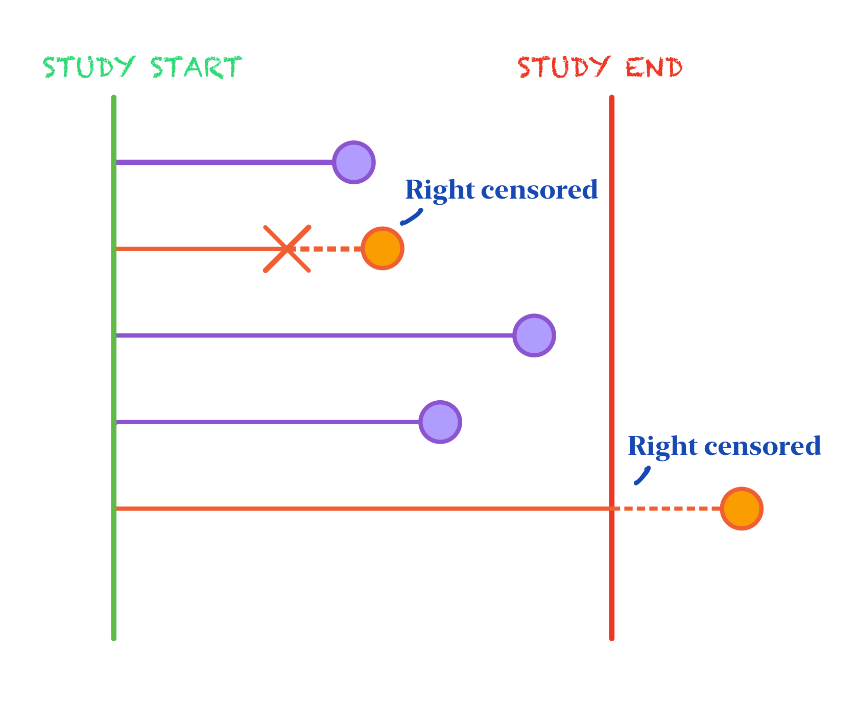
It’s imperative that we still consider these censored observations in our study instead of removing them so that we don’t bias our results towards only those individuals that experienced the event of interest within the observational time frame. Thus, in survival analysis, not only do we include time from baseline at event of interest in our outcome, but we also include a binary variable indicating whether an individual experienced the event or was censored instead.
In standard survival analysis, the survival function, S(t) is what defines the probability that the event of interest has not yet happened at time = t.[4]
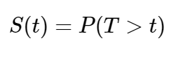
S(t) is non-increasing and ranges between 0 and 1. The hazard function on the other hand is defined as the instantaneous risk of an individual experiencing the event of interest within a small time frame[5].
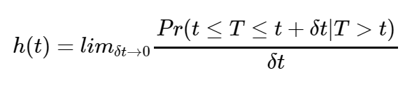
Both survival functions and hazard functions are alternatives to probability density functions and are better suited for survival data.
Survival regression involves not only information about censorship and time to event, but also additional predictor variables of interest like the sex, age, race, etc. of an individual. The Cox proportional hazards model is a popular and widely utilized modeling technique for survival data because it considers the effects of covariates on the outcome of interest as well as examines the relationships between those variables and the survival distribution[6]. While this model is praised for its flexibility and simplicity, it is also often criticized for its restrictive proportional hazards assumption.
The Proportional Hazards Assumption
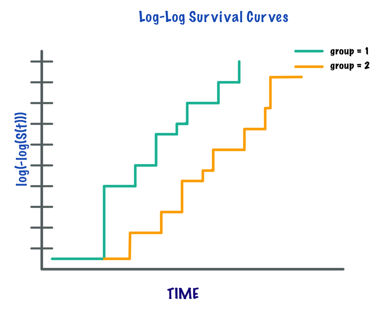
The proportional hazards assumption states that the relative hazard remains constant over time across the different strata/covariate levels in the data[7]. One of the most popular graphical technique for evaluating the PH assumption involves comparing estimated log-log survival curves over different strata of the variables being investigated[8]. A log-log survival curve is a transformation of an estimated survival curve that results from taking the natural log of an estimated survival probability twice. Generally, if the log-log survival curves are approximately parallel for each level of the (categorical) covariates then the proportional hazards assumption is met.
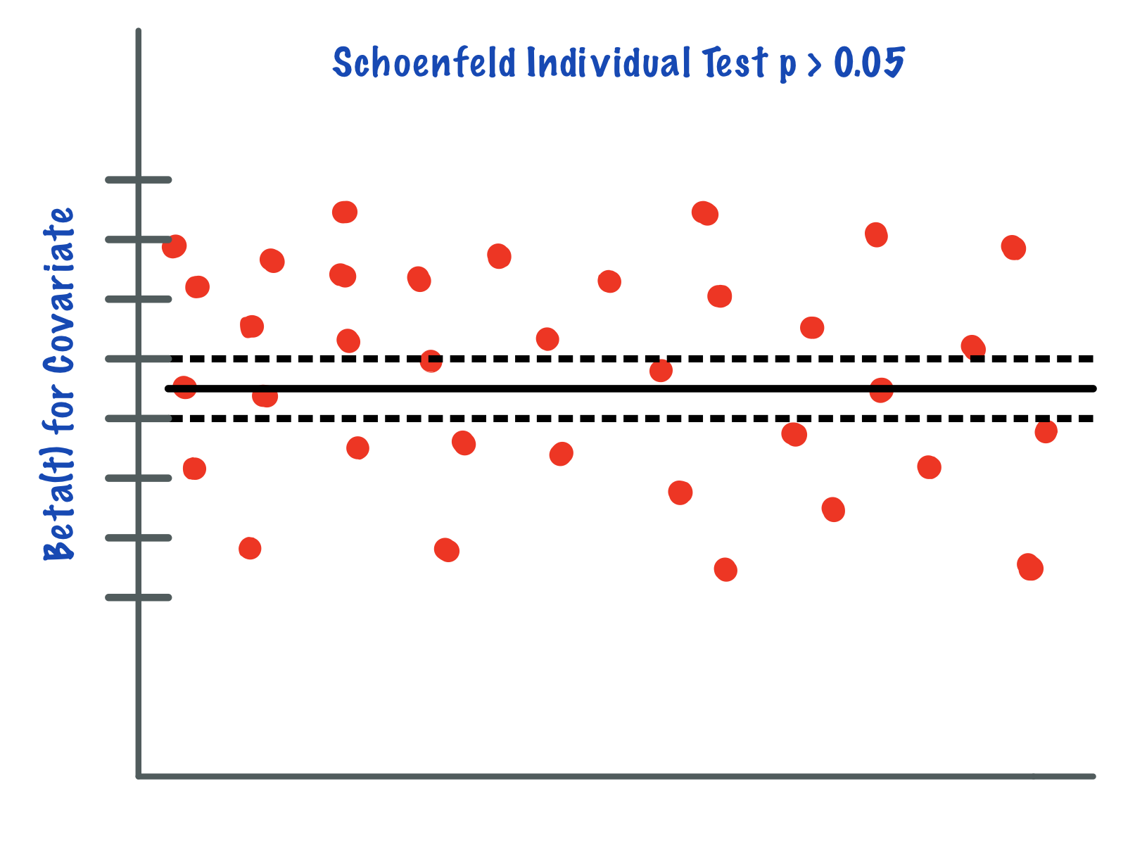
In the case of continuous covariates, this assumption can also be checked using statistical tests and graphical methods based on the scaled Schoenfeld residuals[9]. The Schoenfeld residuals are calculated for all covariates for each individual experiencing an event at a given time. Those are the differences between that individual’s covariate values at the event time and the corresponding risk-weighted average of covariate values among all individuals at risk. The Schoenfeld residuals are then scaled inversely with respect to their covariances/variances. We can think of this as down-weighting the Schoenfeld residuals whose values are unreliable because of high variance. If the assumption is valid, the Schoenfeld residuals are independent of time. A plot that shows a non-random pattern against time is evidence of a violation of the PH assumption. In summary, the proportional hazard assumption is validated by a non-significant (p-value > 0.05) relationship between residuals and time, and disapproved by a significant relationship (p-value ≤ 0.05).
This is a strong assumption and is often viewed as impractical as it is more often than not violated. There are a number of extensions that aim to deal with data that violate this assumption, but they often rely on restrictive functions or limit the ability to estimate the effects of covariates on survival. Random survival forests (RSF) provide an attractive non-parametric alternative to these models[10].
An Extension of Random Forests and Decision Trees
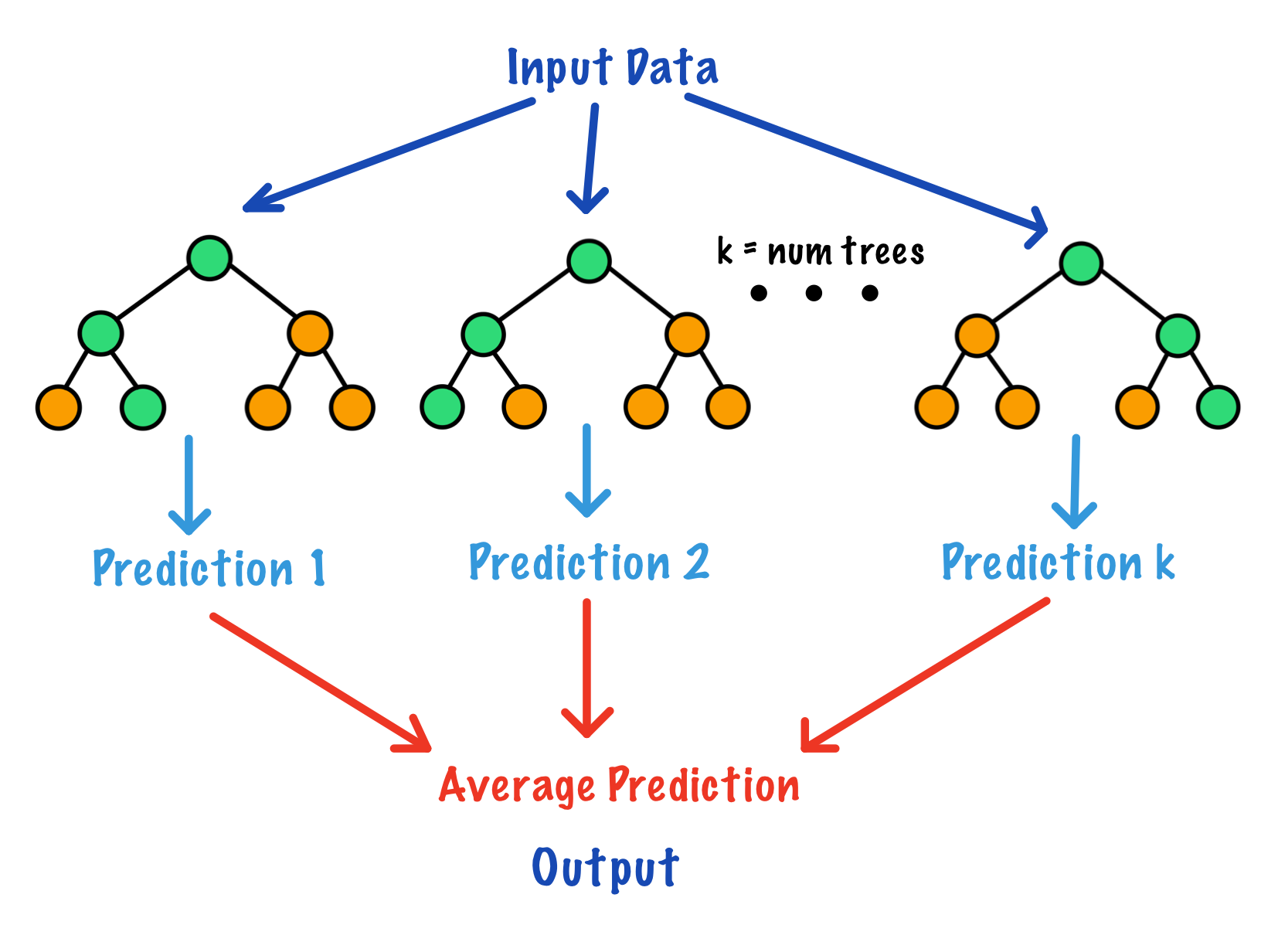
Similar to random forests and decision trees, random survival forests and by extension a method called conditional inference forests (CIF) build trees by recursively partitioning data using binary splits on a set of covariates[11]. Random survival forests provide an alternative approach to the Cox proportional hazards models when the PH assumption is violated. Conditional inference forests reduce selection bias and create partitions using conditional distributions and permutations. These methods are non-parametric, flexible, and used to identify factors in predicting the time-to-event outcome for right-censored survival data.
Random Survival Forests
A random survival forest is an extension of random forests used to analyze time to event right-censored survival data.
Random survival forests use splitting criterion based on survival time and censoring status[12]. Survival trees are binary trees which recursively split tree nodes so that the dissimilarity between child nodes is maximized. Eventually the dissimilar cases are separated and each node becomes more homogeneous. The predictive outcome is defined as the total number of events of interest experienced, which is derived from the ensemble cumulative hazard function (CHF).
The algorithm:
-
Draw B bootstrap samples from the data
-
Grow a survival tree for each bootstrap sample. For each node of the tree, consider p random variables to split on. The node is split with the candidate variable which maximizes the survival difference between child nodes.
-
Grow the tree as long to full size and stop when the terminal node has no less than d0 > 0 unique events.
-
Average over B survival trees to obtain the ensemble CHF.
-
Calculate the prediction error for the ensemble CHF using OOB error.
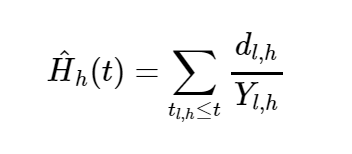
We determine a terminal node h ∈ T when there are no less than d0 > 0 unique events. Let us define dl, h and Yl, h as the number of events and individuals who are at risk at time tl, h. Then the CHF estimate for a terminal node h is defined as
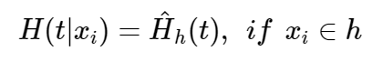
Each individual i has a d dimensional covariate xi. The binary structure of survival trees allows xi to be classified into a unique terminal node h. Thus the CHF for individual i is
The ensemble CHF is found by averaging over
survival trees.
Conditional Inference Forests
While random survival forests tend to be biased toward variables with many split points, conditional inference forests are designed to reduce this selection bias[13]. A conditional inference model is composed of a forest of conditional inference trees. Conditional inference forests are designed by separating the algorithm which selects the best splitting covariate from the algorithm which selects the best split point.
The algorithm:
-
For case weights w, set the global null hypothesis of independence between any of the p covariates and the response variable. Stop the algorithm if we fail to reject the null hypothesis. Otherwise, select the jth covariate Xj* with the strongest association to T.
-
Select a set A* in Xj* in order to split Xj* into two disjoint sets: A* and Xj* without A*. The weights wa and wb determine the two subgroups with
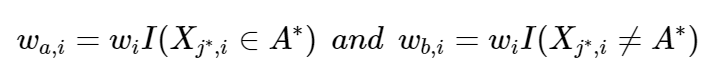
Repeat steps 1 and 2 recursively using modified case-weights wa and wb.
The first step finds the optimal split variable by testing the association of the covariates to the outcome T using a linear rank test. Using permutation tests, the covariate with the strongest association to T is selected for splitting. In the second step, the selection of variables are found using a linear rank test. The covariates with the strongest association to T (i.e. minimum p-value) are used for variable selection.
Applications
We will run a random survival forest model and a conditional inference forest model on two real survival datasets.
PBC Data
The first dataset, the PBC dataset hails from the survival package in
R and summarizes the survival data of 418 primary biliary cirrhosis
(PBC) patients from a randomized trial conducted between 1974 and
1984[14].
Most of the covariates in the PBC data are either continuous or have two levels (few split-points).
Employee Data
The second dataset was found on Kaggle, an online community platform for data scientists and machine learning enthusiasts allowing for the public-use of a vast array of practical datasets. This dataset contains the employee attrition information of 1,129 employees[15].
Unlike the PBC dataset, this data consists of many categorical variables with most of them having more than two-levels (many split-points).
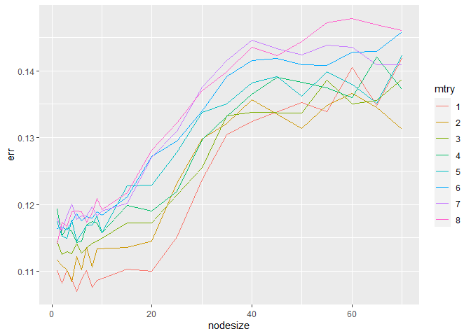
Model Tuning
In the case of the random survival forest model, we will consider tuning for two parameter values, number of variables to possibly split at each node (mtry) and minimum size of terminal node (nodesize). We will choose the combination on each data set that yields the lowest out-of-bag error.
Evaluating the Models: Variable Importance
For each model, we will assess the ranked variable importance. We’ll
do this using the varImp function from the caret package in R[16].
This function tracks the changes in metric statistics for each predictor
and accumulates the reduction in the statistic when each predictor is
added to the model. The reduction is the measure of variable importance.
For trees/forests, the prediction accuracy on the out of bag sample is
recorded. The same is done after permuting each predictor variable. The
difference between the two accuracies are averaged over all trees and
normalized. We’ll aim to compare how each of the two models rank the
importance of the different covariates.
Evaluating the Models: Brier Scores
In comparative studies, it is of interest to measure the predictive accuracy of different survival regression strategies for building a risk prediction model. There are several metrics that can be used to assess the resulting probabilistic risk predictions. We’re going to focus on one of the most popular metrics, the Brier score[17]. The brier score for an individual is defined as the squared difference between observed survival status (1 = censored at time t and 0 = event experienced at time t) and a model based prediction of ‘surviving’ up to time t. The survival status at time t will be right-censored for some data. For time-to-event outcome, this measure can be estimated point-wise over time. We will concentrate on comparing the performance of our models using prediction error curves that are obtained by combining time-dependent estimates of the population average Brier score[18].
Using a test sample of size
, Brier scores at time t are defined as:
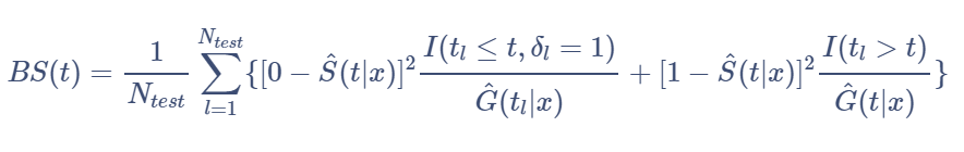
where
P(C > t | X = x) is the Kaplan-Meier estimate of the conditional
survival function of the censoring times.
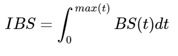
The integrated Brier scores are given by:
To avoid the problem of overfitting that arises from using the same data to train and test the model, we used the Bootstrap cross-validated estimates of the integrated Brier scores[19]. The prediction errors are evaluated in each bootstrap sample.
The prediction errors for each of our models will be implemented in the
pec package in R[20]. We implement bootstrap cross-validation to get
our estimates for the integrated brier scores. The models are assessed
on the data samples that are NOT in the bootstrap sample (OOB data).
PBC Data
The following description comes from the survival package in R[21]:
Primary sclerosing cholangitis is an autoimmune disease leading to destruction of the small bile ducts in the liver. Progression is slow but inexorable, eventually leading to cirrhosis and liver decompensation.
This data is from the Mayo Clinic trial in PBC conducted between 1974 and 1984. A total of 424 PBC patients met eligibility criteria for the randomized placebo controlled trial of the drug D-penicillamine. This dataset tracks survival status until end up follow up period as well as contains many covariates collected during the clinical trial.
| Variable | Description |
|---|---|
| id | case number |
| time | number of days between registration and the earlier of death, transplant, or end of observational period |
| status | status at endpoint, 0/1/2 for censored, transplant, dead |
| trt | 1/2/NA for D-penicillmain, placebo, not randomized |
| age | in years |
| sex | m/f |
| ascites | presence of ascites |
| hepato | presence of hepatomegaly or enlarged liver |
| spiders | blood vessel malformations in the skin |
| edema | 0 no edema, 0.5 untreated or successfully treated 1 edema despite diuretic therapy |
| bili | serum bilirunbin (mg/dl) |
| chol | serum cholesterol (mg/dl) |
| albumin | serum albumin (g/dl) |
| copper | urine copper (ug/day) |
| alk.phos | alkaline phosphotase (U/liter) |
| ast | aspartate aminotransferase, once called SGOT (U/ml) |
| trig | triglycerides (mg/dl) |
| platelet | platelet count |
| protime | standardized blood clotting time |
| stage | histologic stage of disease (needs biopsy) |
Variable Selection
In order to choose the variables that we want to use in our models, we will first run a cox proportional hazards model with all of the possible main effects in our data. We will then go through a backwards elimination process, removing the variables with the highest p-values over a significance level of 0.05 one by one until all of the main effects are statistically significant. Then, we’ll test for all two-way interaction terms and perform backwards elimination until all two-way interactions left in the model are statistically significant.
Note that the status variable will be simplified to two levels. Individuals will have a value of 1 if they experienced death and 0 otherwise, making death our event of interest.
# test main effects
pbc.main <- coxph(Surv(time, status) ~ ., data =  pbc_use)
step(pbc.main, direction = "backward")

# test two-way interactions
pbc.full <- coxph(Surv(time, status) ~ (.)^2, data =  pbc_use)
#step(pbc.full, direction = "backward")
Going through backwards elimination leaves us with a model with age, edema status (edema), serum bilirunbin (bili), serum albumin (albumin), urine copper (copper), aspartate aminotransferase (ast), standardized blood clotting time (protime), histologic stage of disease (stage) and the interactions between age and edema status, age and urine copper, and serum bilirunbin and aspartate aminotransferase.
Note that due to the nature of this dataset, some of the subgroups have not yet reached 50% survival as far as the scope of the information that we have goes. Thus, some survival times were not able to be implemented by our methods due to ‘missingness’. To make up for this shortage, we utilized an oversampling technique to bootstrap sample for more observations which also ended up sampling for more censored observations in our data.
pbc_cox <- coxph(Surv(time, status) ~ age + edema + bili + albumin +
  copper + ast + protime + stage + age:edema + age:copper +
  bili:ast,
  data = pbc_use)
We can test the proportional-hazards assumption using the cox.zph
function.
For each covariate, the function correlates the corresponding set of scaled Schoenfeld residuals with time to test for independence between residuals and time. Additionally, it performs a global test for the model as a whole.
test.ph <- cox.zph(pbc_cox)
test.ph

##             chisq df       p
## age        10.884  1 0.00097
## edema       1.115  1 0.29091
## bili        6.809  1 0.00907
## albumin     3.630  1 0.05673
## copper      0.932  1 0.33430
## ast         0.716  1 0.39761
## protime    14.552  1 0.00014
## stage      17.315  1 3.2e-05
## age:edema   1.053  1 0.30492
## age:copper  0.292  1 0.58908
## bili:ast   11.955  1 0.00055
## GLOBAL     63.669 11 1.9e-09
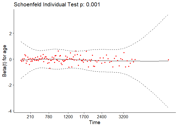
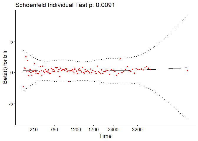
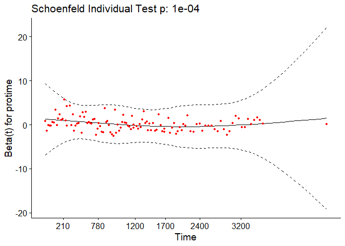
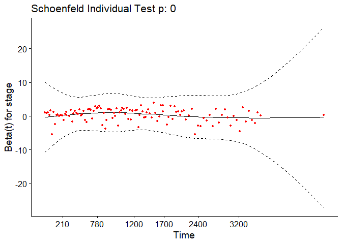
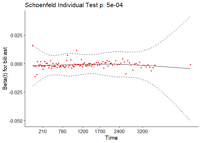
The output from the test tells us that the test is statistically significant for age, bili, protime, stage, and the interaction between bili and ast at a significance level of 0.05. It’s also globally statistically significant with a p-value of 2e-09. Thus, the PH assumption is violated.
Using random survival forests and conditional inference forests are useful alternatives in this case.
Random Survival Forest Implementation
In hyperparameter tuning, which was done using the tune function from
the e1071 package in R, we found that an mtry value of 1 and a
nodesize of 5 produced the lowest out-of-bag error (0.107)[22]. The
random forest model was run using the rfsrc function in the
randomForestSRC package in R[23].
set.seed(1)
# random forest
pbc_rf <- rfsrc(Surv(time, status) ~ age + edema + bili + albumin +
  copper + ast + protime + stage + age:edema + age:copper +
  bili:ast,
  mtry = 1,
  nodesize = 5,
  data = pbc_use)
Conditional Inference Forest Implementation
We build a conditional inference forest using the pecCforest function
from the pec package in R[24].
set.seed(1)
# run conditional inference forest

pbc_cif <- pecCforest(Surv(time, status) ~ age + edema + bili + albumin +
  copper + ast + protime + stage + age:edema + age:copper +
  bili:ast,
  data = pbc_use)
Comparing the Models
We can plot the predicted survival curves for 4 random individuals in our data (2 censored and 2 non-censored) and compare the predicted median survival times (the time where the probability of survival = 0.5 of both of the models) to what is observed.
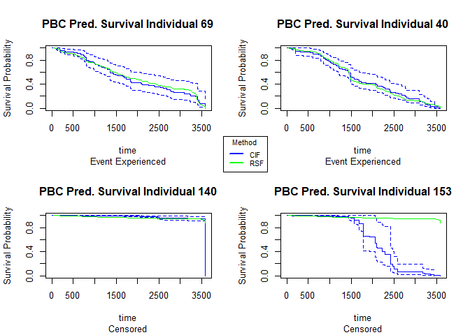
| id | time | event | RSF median survival | CIF median survival |
|---|---|---|---|---|
| 69 | 3395 | 1 | 1827 | 1741 |
| 40 | 1487 | 1 | 1487 | 1536 |
| 140 | 3445 | 0 | 3584 | 3584 |
| 153 | 2224 | 0 | 3584 | 3584 |
For the observations that experienced death, the random forest model predicts a median survival time closer to time of death than the random survival forest model does. For the censored individuals #140 and #153, both models predict the same median survival times for both observations.
Variable Importance
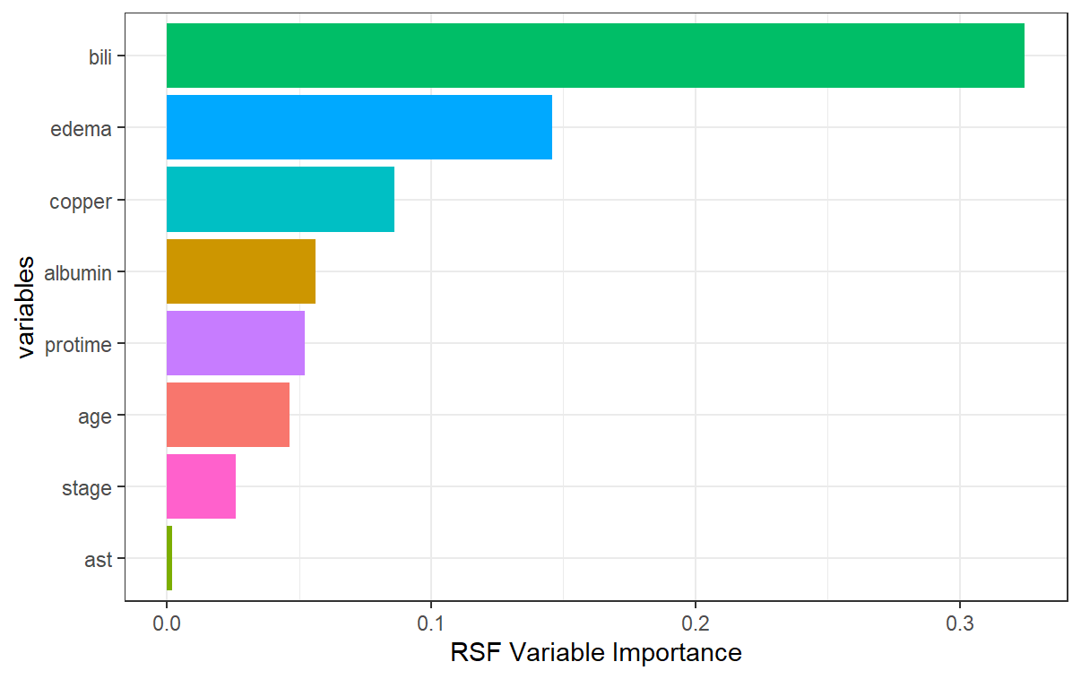
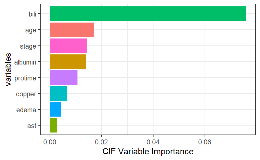
We can compare the variable importance rankings between the random survival forest and the conditional inference forest. Most notably, the scale of variable importance is larger in the conditional inference forest case than it is in the random survival forest. This is because even though bili is the most important predictor in both models, it is that much more important in the conditional inference forest. Additionally, we see that while edema and copper are 2nd and 3rd most important in the random survival forest, they are relatively not that important in the conditional inference forest. Conversely, while age and stage are important in the conditional inference forest, they are not as important in the random survival forest. One thing to note is that the variable edema can be viewed as a predictor with many split-points (greater than 2), taking on three unique values: 0, 0.5, and 1. We may be seeing the inherent bias problem coming into play here in the fact that the random survival forest favors that variable in terms of its importance.
Prediction Error Curves
We can compare the prediction error curves for the random survival forest and the conditional inference forest models.
Using bootstrap cross-validation (
=
50), we see an integrated brier score of 0.068 for the random survival
forest and 0.073 for the conditional inference forest. Recall that a
lower score means better performance. While the random survival forest
performs better here, the difference is marginal and perhaps negligible.
##
## Integrated Brier score (crps):
##
##         AppErr BootCvErr
## rsf      0.041     0.068
## cforest  0.055     0.073
Employee Turnover Data
A dataset found on Kaggle containing the employee attrition information of 1,129 employees and information about time to turnover, their gender, age, industry, profession, employee pipeline information, the presence of a coach on probation, the gender of their supervisor, and wage information.
| Variable | Description |
|---|---|
| stag | Experience (time) |
| event | Employee turnover |
| gender | Employee’s gender, female (f), or male (m) |
| age | Employee’s age (year) |
| industry | Employee’s Industry |
| profession | Employee’s profession |
| traffic | From what pipeline employee came to the company. 1. contacted the company directly (advert). 2. contacted the company directly on the recommendation of a friend that’s not an employee of the company (recNErab). 3. contacted the company directly on the recommendation of a friend that IS an employee of the company (referral). 4. applied for a vacancy on the job site (youjs) 5. recruiting agency brought you to the employer (KA) 6. invited by an employer known before employment (friends). 7. employer contacted on the recommendation of a person who knows the employee (rabrecNErab). 8. employer reached you through your resume on the job site (empjs). |
| coach | presence of a coach (training) on probation |
| head_gender | head (supervisor) gender (m/f) |
| greywage | The salary does not seem to the tax authorities. Greywage in Russia or Ukraine means that the employer (company) pay just a tiny bit amount of salary above the white-wage (white-wage means minimum wage) (white/gray) |
| way | Employee’s way of transportation (bus/car/foot) |
| extraversion | Extraversion score |
| independ | Independend score |
| selfcontrol | Self-control score |
| anxiety | Anxiety Score |
| novator | Novator Score |
Variable Selection
We’ll follow the same variable selection procedure that we did for the PBC data.
# test main effects
turn.main <- coxph(Surv(stag, event) ~ ., data =  turn_use)
step(turn.main, direction = "backward")

# test two-way interactions
turn.full <- coxph(Surv(stag, event) ~ (.)^2, data =  turn_use)
step(turn.full, direction = "backward")
Going through backwards elimination leaves us with a model with age, employee’s industry (industry), employee’s profession (profession), employee’s pipeline origin (traffic), wage standard (greywage), employee’s way of transportation (way), self-control score (selfcontrol), anxiety score (anxiety), and the interactions between age and way of transportation and way of transportation and self-control score.
turn_cox <- coxph(Surv(stag, event) ~ age + industry + profession + traffic +
        greywage + way + selfcontrol + anxiety + age:way + way:selfcontrol,
       data =  turn_use)
We can test the proportional-hazards assumption for this model using the
cox.zph function.
test.ph_turn <- cox.zph(turn_cox)
test.ph_turn

##                   chisq df       p
## age              1.9060  1 0.16741
## industry        21.6544 15 0.11719
## profession      40.4758 14 0.00021
## traffic         11.9480  7 0.10228
## greywage         1.2658  1 0.26055
## way              1.0839  2 0.58160
## selfcontrol      0.0687  1 0.79319
## anxiety          1.0692  1 0.30112
## age:way          2.5780  2 0.27554
## way:selfcontrol  0.6640  2 0.71750
## GLOBAL          73.0448 46 0.00677

The output from the test tells us that the test is statistically significant for profession at a significance level of 0.05. It’s also globally statistically significant with a p-value of 0.007. Thus, the PH assumption is violated and random survival forests and conditional inference forests can be useful alternatives with this data as well.
Random Survival Forest Implementation
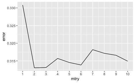
In hyperparameter tuning which was done by changing mtry values using
the ranger function from the ranger package in R, we found that an
mtry value of 2 produced the lowest out-of-bag error (0.313)[25].
Note that to run random survival forest for the employee turnover data,
due to computational issues, we’ve switched to using the ranger
function as opposed to the rfsrc function. We’ll run a parameter tuned
random survival forest model with the variables and interactions that we
identified in variable selection.
set.seed(1)
# random survival forest
turn_rsf <- ranger(Surv(stag, event) ~ age + industry + profession + traffic +
        greywage + way + selfcontrol + anxiety +
          age.way + way.selfcontrol,
        mtry = 2,
       data =  turn_use)
Conditional Inference Forest Implementation
We’ll run a conditional inference forest model next with the variables and interactions that we identified in variable selection.
set.seed(1)
turn_cif <- pecCforest(Surv(stag, event) ~ age + industry + profession + traffic +
        greywage + way + selfcontrol + anxiety +
          age.way + way.selfcontrol,
       data =  turn_use)
Comparing the Models
Similar to the PBC data, we will choose 4 random individuals in the study, 2 who experienced the event of interest and 2 who are censored, and plot and compare their predicted survival curves as well as their predicted median survival times ( the time where the probability of survival = 0.5) to what is observed.
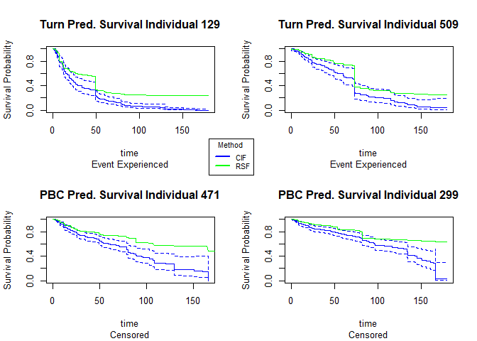
| id | time | event | RSF median survival | CIF median survival |
|---|---|---|---|---|
| 129 | 49.38 | 1 | 49.3 | 21.6 |
| 509 | 73.3 | 1 | 74.1 | 73.3 |
| 471 | 14.49 | 0 | 164.6 | 80.2 |
| 299 | 73.43 | 0 | 179.4 | 133.0 |
For the observations that experienced death, the random forest model predicts a median survival time closer to time of death than the conditional inference forest model does. For the censored individuals, the conditional inference forest model predicts small median survival times that occur within the course of the study.
Variable Importance
We’ll compare the variables that the random survival forest model and the conditional inference forest model found to be most important in the training process on the employee turnover data.
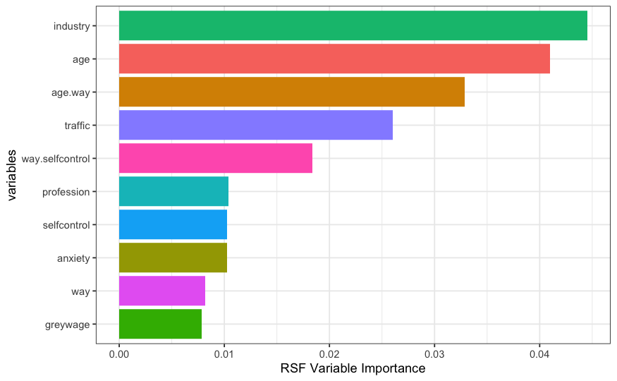
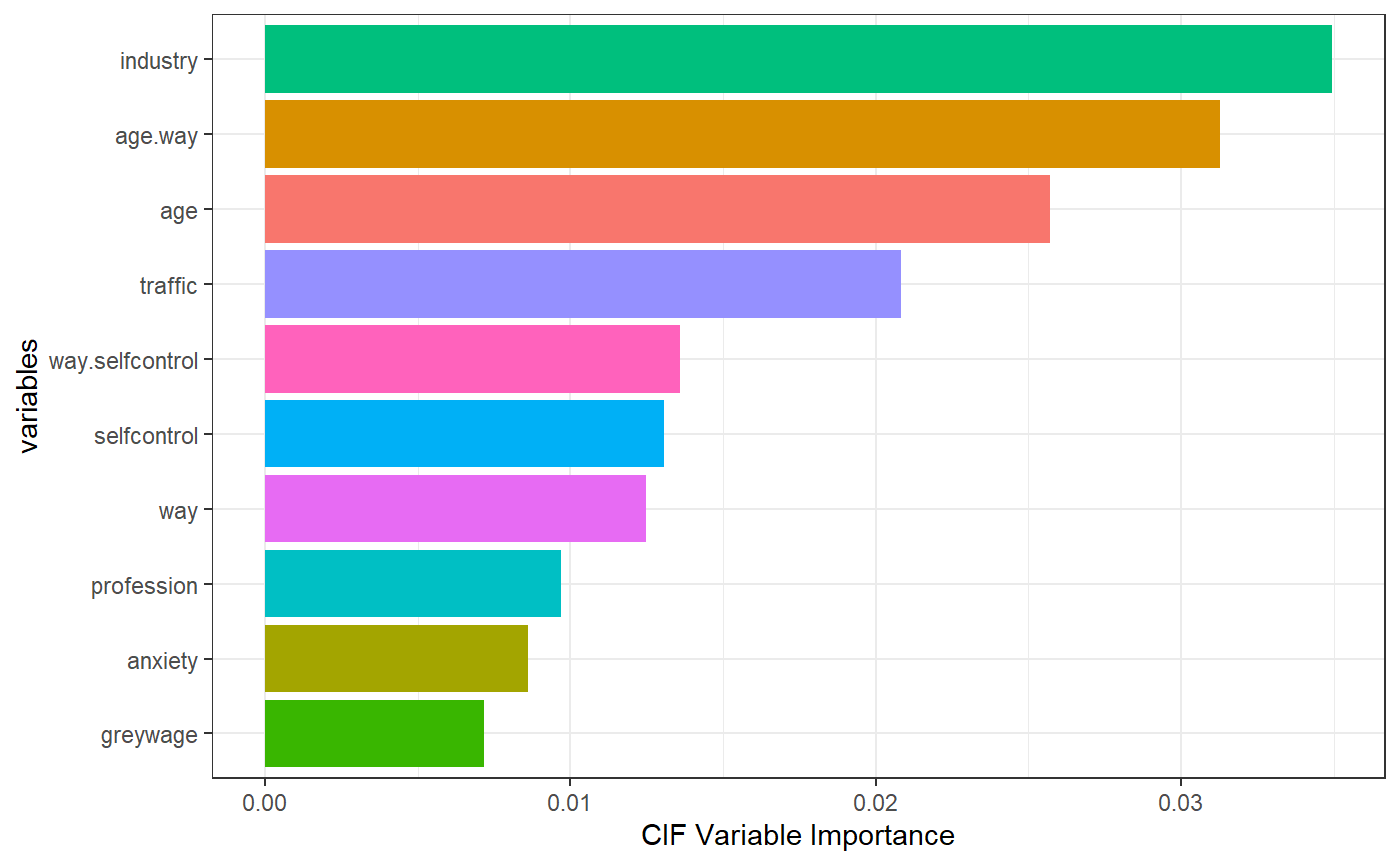
While the two models generally agree on the first 5 most important variables (with a switch in age and age.way in terms of order), we can focus on the magnitude of the variable importance as well as the ordering of variables ranked 6-9. The industry variable in the dataset is one of the variables that has the most split points/levels. There are 16 unique variables that industry can take. Even though both models rank this variable to be the most important, relative to the conditional inference forest, the random survival forest seems to slightly inflate the importance of this covariate as it reaches an importance of just over 0.04 in the random survival forest (as opposed to about 0.035 in the conditional inference forest). After the first 5 variables, the random survival forest ranks profession, self-control, anxiety, and way as the next important while the conditional inference forest ranks self-control, way, profession, and then anxiety as the next important.
What may be of interest here is the ranking of the profession variable which has 15 unique split points. The random survival forest ranks this variable 2 places higher than the conditional inference forest does. The conditional inference forest on the other hand seems to favor the continuous self-control score over profession which may indicate an attempt to control for bias.
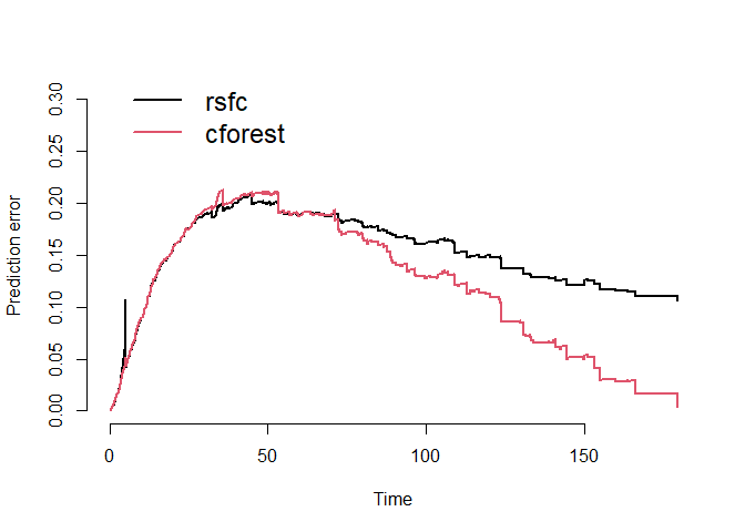
Prediction Error Curves
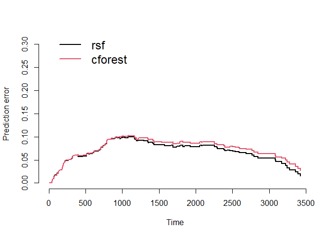
We can compare the prediction error curves of the two models. Recall
that these estimates are based on the average brier scores computed at
different time points. We reduce to
= 5
for computation and run-time purposes. Using bootstrap cross-validation,
we see an integrated brier score of 0.15 for the random survival forest
and 0.12 for the conditional inference forest. Thus, in the case of this
employee turnover data, the conditional inference forest performs
noticeably better than the random survival forest, especially as time
increases.
##
## Integrated Brier score (crps):
##
##         AppErr BootCvErr
## rsfc     0.082      0.15
## cforest  0.061      0.12
Closing Thoughts
In summary, we observed that while both random survival forests and conditional inference forests performed well when predicting the time to death and employee turnover within two separate datasets, the conditional inference forest seemed to perform notably better in the face of categorical covariates with many split-points. This result may suggest that conditional inference forests tend to be better suited to adjust for the bias that random survival forests struggle with when there are multi-leveled predictors in our data. However, in the case of covariates with few split-points, the two models seem to perform comparatively. Therefore, we can be reinforced of the importance of exploratory data analysis and its contribution to the choice of an appropriate model to analyze our data. Ultimately, random survival forests and conditional inference forests are two of many robust models for the analysis of time-to-event data. Further studies may take an interest in learning more about these alternative modeling techniques, including those that take a Bayesian approach in the applications of these data.
References:
[1] Goel, M. K., Khanna, P., & Kishore, J. (2010). Understanding survival analysis: Kaplan-Meier estimate. International journal of Ayurveda research, 1(4), 274.
[2] Goel, M. K., Khanna, P., & Kishore, J. (2010). Understanding survival analysis: Kaplan-Meier estimate. International journal of Ayurveda research, 1(4), 274.
[3] Prinja, S., Gupta, N., & Verma, R. (2010). Censoring in clinical trials: review of survival analysis techniques. Indian journal of community medicine: official publication of Indian Association of Preventive & Social Medicine, 35(2), 217.
[4] Kleinbaum, D. G., & Klein, M. (2012). Survival analysis: a self-learning text (Vol. 3). New York: Springer.
[5] Kleinbaum, D. G., & Klein, M. (2012). Survival analysis: a self-learning text (Vol. 3). New York: Springer.
[6] Kleinbaum, D. G., & Klein, M. (2012). The Cox proportional hazards model and its characteristics. In Survival analysis (pp. 97-159). Springer, New York, NY.
[7] Kleinbaum, D. G., & Klein, M. (2012). The Cox proportional hazards model and its characteristics. In Survival analysis (pp. 97-159). Springer, New York, NY.
[8] Sestelo, M. (2017). A short course on Survival Analysis applied to the Financial Industry.
[9] Hess, K. R. (1995). Graphical methods for assessing violations of the proportional hazards assumption in Cox regression. Statistics in medicine, 14(15), 1707-1723.
[10] Nasejje, J. B., Mwambi, H., Dheda, K., & Lesosky, M. (2017). A comparison of the conditional inference survival forest model to random survival forests based on a simulation study as well as on two applications with time-to-event data. BMC medical research methodology, 17(1), 1-17.
[11] Nasejje, J. B., Mwambi, H., Dheda, K., & Lesosky, M. (2017). A comparison of the conditional inference survival forest model to random survival forests based on a simulation study as well as on two applications with time-to-event data. BMC medical research methodology, 17(1), 1-17.
[12] Nasejje, J. B., Mwambi, H., Dheda, K., & Lesosky, M. (2017). A comparison of the conditional inference survival forest model to random survival forests based on a simulation study as well as on two applications with time-to-event data. BMC medical research methodology, 17(1), 1-17.
[13] Nasejje, J. B., Mwambi, H., Dheda, K., & Lesosky, M. (2017). A comparison of the conditional inference survival forest model to random survival forests based on a simulation study as well as on two applications with time-to-event data. BMC medical research methodology, 17(1), 1-17.
[14] Therneau, T. M. (2020). A Package for Survival Analysis in R. https://CRAN.R-project.org/package=survival
[15] Wijaya, D. (2020, September 5). Employee Turnover. Kaggle. Retrieved May 14, 2022, from https://www.kaggle.com/datasets/davinwijaya/employee-turnover?select=turnover.csv
[16] Kuhn, M. (2008). Building Predictive Models in R Using the caret Package. Journal of Statistical Software, 28(5), 1 - 26. doi:http://dx.doi.org/10.18637/jss.v028.i05
[17] Nasejje, J. B., Mwambi, H., Dheda, K., & Lesosky, M. (2017). A comparison of the conditional inference survival forest model to random survival forests based on a simulation study as well as on two applications with time-to-event data. BMC medical research methodology, 17(1), 1-17.
[18] Mogensen, U. B., Ishwaran, H., & Gerds, T. A. (2012). Evaluating random forests for survival analysis using prediction error curves. Journal of statistical software, 50(11), 1.
[19] Nasejje, J. B., Mwambi, H., Dheda, K., & Lesosky, M. (2017). A comparison of the conditional inference survival forest model to random survival forests based on a simulation study as well as on two applications with time-to-event data. BMC medical research methodology, 17(1), 1-17.
[20] Mogensen UB, Ishwaran H, Gerds TA (2012). “Evaluating Random Forests for Survival Analysis Using Prediction Error Curves.” Journal of Statistical Software, 50(11), 1–23. https://www.jstatsoft.org/v50/i11.
[21] Therneau, T. M. (2020). A Package for Survival Analysis in R. https://CRAN.R-project.org/package=survival
[22] Meyer D, Dimitriadou E, Hornik K, Weingessel A, Leisch F
(2021). _e1071: Misc Functions of the Department of
Statistics, Probability Theory Group (Formerly: E1071), TU
Wien_. R package version 1.7-9,
https://CRAN.R-project.org/package=e1071.
[23] Ishwaran H. and Kogalur U.B. (2022). Fast Unified Random Forests for Survival,
Regression, and Classification (RF-SRC), R package version 3.1.0.
[24] Ulla B. Mogensen, Hemant Ishwaran, Thomas A. Gerds (2012). Evaluating Random
Forests for Survival Analysis Using Prediction Error Curves. Journal of
Statistical Software, 50(11), 1-23. DOI 10.18637/jss.v050.i11
[25] Marvin N. Wright, Andreas Ziegler (2017). ranger: A Fast Implementation of
Random Forests for High Dimensional Data in C++ and R. Journal of Statistical
Software, 77(1), 1-17. <doi:10.18637/jss.v077.i01>